How To Draw A Horizontal Line In Google Chart

Adding a goal/target line across a cavalcade chart is non a tough job. With a combo chart, anyone can easily exercise it in Google Sheets. Y'all just want to know how to format the data to include the goal/target value.

With just one additional column with your source data, you tin add a goal line to your nautical chart. I am going to explicate that in detail here.

In this tutorial, I accept additionally included a dynamic chart. In that, I have used a data validation drop-downwardly menu to dynamically switch the monthly data and monthly targets.

I volition come back to this later. Starting time, yous must know what is a target line or goal line in column charts.

Understand the Target / Goal Line in Column Chart in Google Sheets

When you have set a stock-still target or goal for multiple categories it's a good idea to visualize that data with a column chart. In such charts, y'all tin can draw a directly target line across the nautical chart.

For case, I gave the aforementioned targets for my different salespeople. I tin can compare their performance based on the given fixed target.

With a cavalcade chart that contains a target line beyond, I can hands understand who has come upwards to my expectation.

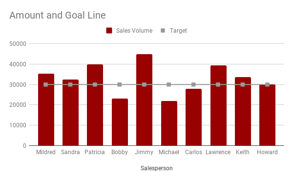
See the target line across the column chart. Each cavalcade shows the sales volume for each salesperson. The horizontal straight line is the target gear up for them.

From this, you lot can easily pick the salespersons who are under performing. As you can see they are "Bobby", "Michael" and "Carlos".

I will give step-past-step instructions to how to add together a target line beyond a column chart as higher up in Google Sheets. Before that meet this dynamic column chart with the goal line added.

Actually, the goal line is muted. Instead, I preferred to show the data square point to improve the visual appearance of my chart.

Horizontal goal data points in column chart

The above chart shows the monthly target of each salesperson and their performance.

How to Add a Target Line Across a Column Chart in Google Sheets

I have shown you ii charts – one basic chart with horizontal target line and another dynamic chart with data points instead of a line. Let me outset with the first nautical chart.

Create a Bones Column Chart with Horizontal Target Line in Sheets

Enter the sample information as below.

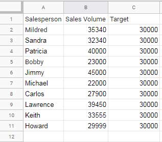
Formatted data for basic column chart with target line

Y'all tin get the finished chart with the in a higher place sample data hither. You can become that or type the above sample data equally shown.

In this sample data, the tertiary column contains the target value which should be the aforementioned in each and every row.

Steps to Create the Column Chart with Goal Line:

Select the information in A1:C. Then open the chart editor.

You can admission the chart editor sidebar panel from the menu Insert > Chart.

In the chart editor panel, select the chart type as "Combo chart", which is important.

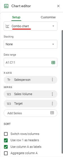
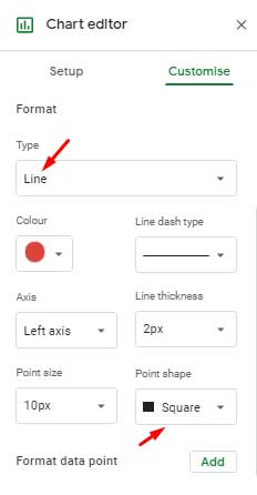
The exact settings should be as in a higher place. Then click on the "Customize" tab on the chart editor.

Click "Serial". Select the serial "Sales book" and set it to "Column", if already not. And so select "Target" and set it to "Line". So change the information point shape to "Square".

This manner y'all can get a target line across a cavalcade nautical chart.

Get a Dynamic Column Chart with Target Data Points in Sheets

Over again you should follow all the above steps. The only deviation is nosotros are populating the source data to plot the chart with a formula.

I have the beneath Kickoff + Match combination formula in cell B2 to extract the data 'dynamically' from the range H2:One thousand.

          =offset(H2:M,0,match(F2,H1:M1,0)-1,COUNT(H2:H),2)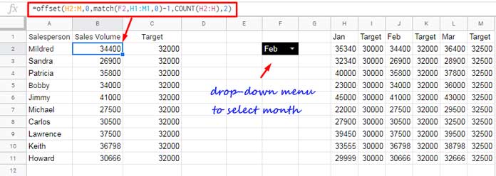

Column A contains the names of salespersons and their monthly sales and targets are shown in the columns H to Grand.

The Offset + Match combination formula (there is Count too) extracts the values from H2:Thou based on the value in jail cell F2 (drib-down bill of fare).

Formula Logic and Explanation:

To understand this formula, I think information technology's better to get thru' the Offset office syntax.

          OFFSET(cell_reference, offset_rows, offset_columns, [elevation], [width])

As per my formula;

offset_rows: 0 – we don't want to commencement any rows. What we want is to offset columns.

offset_columns: Here I have used the Match formula. It uses the search key in jail cell F2 to find its position in the range H1:M1.

If the search key is "Jan", the formula will return # i. It represents the first column. So I have put -1 to make it 0. Otherwise, the Offset will offset 1 column.

height: It's the number of rows to return. Here I accept used the Count function to count the rows in our source data.

width: 2 – Information technology is the number of columns to return. It's two considering I want the sales volume cavalcade and the corresponding target value cavalcade.

In prison cell F2, I have a drop-down with the month proper name as the menu items. It'due south the search key in Friction match to dynamically first the columns.

That drib-down you can create as below.

Go to the menu Information and cull Data validation.
Set the settings equally below.

In this dynamic column nautical chart, I have muted the horizontal target line. That yous tin do by changing the line thickness to 0px of the series "Target". This y'all can find under the chart editor customize tab, series, Target.

That's all. Enjoy!

Additional Resources: